Date last run: 10Oct2020
Load packages that will be used
HOQCutil::silent_library(c('knitr','tidyr','ggplot2'))
Introduction
The Dutch healthcare system repays insured individuals the costs they have made for health reasons. Of course there are lots of details but
the article Understanding ‘Eigen Risico’ gives an introduction.
Only costs above a certain amount (the excess that is called ‘eigen risico’ in Dutch) are repaid. The standard excess is 385 euros but an individual can choose a regime with an higher amount and is then compensated by a reduction of the premium according to Table 1:
er  <- 285+100*(1:6)
pr  <- -48 + 48*(1:6)
| regime | excess | reduction |
|---|---|---|
| 1 | 385 | 0 |
| 2 | 485 | 48 |
| 3 | 585 | 96 |
| 4 | 685 | 144 |
| 5 | 785 | 192 |
| 6 | 885 | 240 |
Net amount to pay for health costs
For each gross amount each regime has a corresponding net amount:
net_amount <- function (gross_amount,regime) {
  er1 = er[regime]
  pr1 = pr[regime]
  pmin(gross_amount,er1) - pr1
}
Calculate net amount for gross amount in the range [0, 1000] for each regime
The function fun calculates the net amounts for one regime and y contains these for all regimes in a list. The results are placed in data.frame df1.
gross_amounts <- seq.int(0,1000,5)
fun <- function (regime) {
  purrr::map_dbl(gross_amounts,~net_amount(.,regime))
}
y <- purrr::map(1:6,fun)
df1 <- data.frame(
  x=gross_amounts,
  er385= y[[1]], er485= y[[2]], er585= y[[3]],
  er685= y[[4]], er785= y[[5]], er885= y[[6]]
)
Create plot after making data.frame ‘long’
The columns with names starting with ‘er’ are then ‘gathered’ in the field ownrisk where these characters are omitted
df1L <-tidyr::pivot_longer(df1,er385:er885,names_to='ownrisk',names_pattern='er(.*)' )
p=ggplot(data=df1L,aes(x,value,group=ownrisk,color=ownrisk,linetype=ownrisk)) +
  geom_line(size=1) +
  labs( caption = "Data source: Zilveren Kruis",
        x="gross amount", y = "net amount") +
  theme(
    plot.title = element_text(hjust = 0.5),
    plot.subtitle = element_text(hjust = 0.5)
)
p

Conclusion
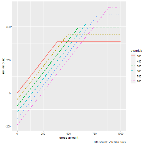
From Figure 1 we see that despite the existence of the various regimes there are only two optimal regimes:
- regime 6 (excess amount 885) when the gross amount is less or equal than 625. For
gross amount = 625the net amount is 625 - 240 = 385 - regime 1 (excess amount 385) when the gross amount is greater or equal than 625. For
gross amount = 625the net amount is 385 - 0 = 385
So the problem of determining an optimal excess amount (eigen risico) is reduced to estimating beforehand if the gross amount is more or less than 625 euros in a year.
Session Info
This document was produced on 10Oct2020 with the following R environment:
  #> R version 4.0.2 (2020-06-22)
  #> Platform: x86_64-w64-mingw32/x64 (64-bit)
  #> Running under: Windows 10 x64 (build 18363)
  #>
  #> Matrix products: default
  #>
  #> locale:
  #> [1] LC_COLLATE=English_United States.1252
  #> [2] LC_CTYPE=English_United States.1252
  #> [3] LC_MONETARY=English_United States.1252
  #> [4] LC_NUMERIC=C
  #> [5] LC_TIME=English_United States.1252
  #>
  #> attached base packages:
  #> [1] stats     graphics  grDevices utils     datasets  methods   base
  #>
  #> other attached packages:
  #> [1] ggplot2_3.3.2 tidyr_1.1.2   knitr_1.30
  #>
  #> loaded via a namespace (and not attached):
  #>  [1] magrittr_1.5     munsell_0.5.0    tidyselect_1.1.0 HOQCutil_0.1.24
  #>  [5] colorspace_1.4-1 R6_2.4.1         rlang_0.4.7      highr_0.8
  #>  [9] stringr_1.4.0    dplyr_1.0.2      tools_4.0.2      grid_4.0.2
  #> [13] gtable_0.3.0     xfun_0.17        withr_2.2.0      htmltools_0.5.0
  #> [17] ellipsis_0.3.1   digest_0.6.25    tibble_3.0.3     lifecycle_0.2.0
  #> [21] crayon_1.3.4     farver_2.0.3     captioner_2.2.3  purrr_0.3.4
  #> [25] vctrs_0.3.4      glue_1.4.2       evaluate_0.14    rmarkdown_2.4
  #> [29] labeling_0.3     stringi_1.5.3    compiler_4.0.2   pillar_1.4.3
  #> [33] scales_1.1.1     generics_0.0.2   pkgconfig_2.0.3