Open Street Map vectors in R (part1)

Date last run: 01Jul2020

Introduction

Here we show how to use Open Street Map vector data to create a map

Load the necessary libraries

HOQCutil::silent_library(c('sf','osmdata', 'ggplot2', 
                           'dplyr','purrr','stringr'))

Read in Open Street Map vector data in given bbox

We read all vector data in a (not so) arbitrary environment in the list od. The elements with names starting with ‘osm_’ contain features of the indicated type. We will list the number of features in each of them but will only consider now the ‘polygons’. We start by making a plot

bbox = c (4.863, 52.307, 4.867, 52.311)
q =	
  osmdata::opq(bbox = bbox) %>%
  osmdata::add_osm_feature(key="^.*$", value="^.*$",
                           key_exact = FALSE,value_exact = FALSE) 
od = osmdata::osmdata_sf (q) 
names(od)
#> [1] "bbox"              "overpass_call"     "meta"             
#> [4] "osm_points"        "osm_lines"         "osm_polygons"     
#> [7] "osm_multilines"    "osm_multipolygons"
odf = purrr::keep(od,stringr::str_detect(names(od),'^osm_'))
odf = purrr::map(odf,~nrow(.))
unlist(purrr::map_if(odf,purrr::map_lgl(odf,is.null),~0))
#>        osm_points         osm_lines      osm_polygons    osm_multilines 
#>              4635               292               548                 4 
#> osm_multipolygons 
#>                 0

# Show the fetched polygons
ggplot() +
  geom_sf(data=od$osm_polygons)

plot of chunk polygons_rough

Figure 1: Open Street Map polygons in bbox

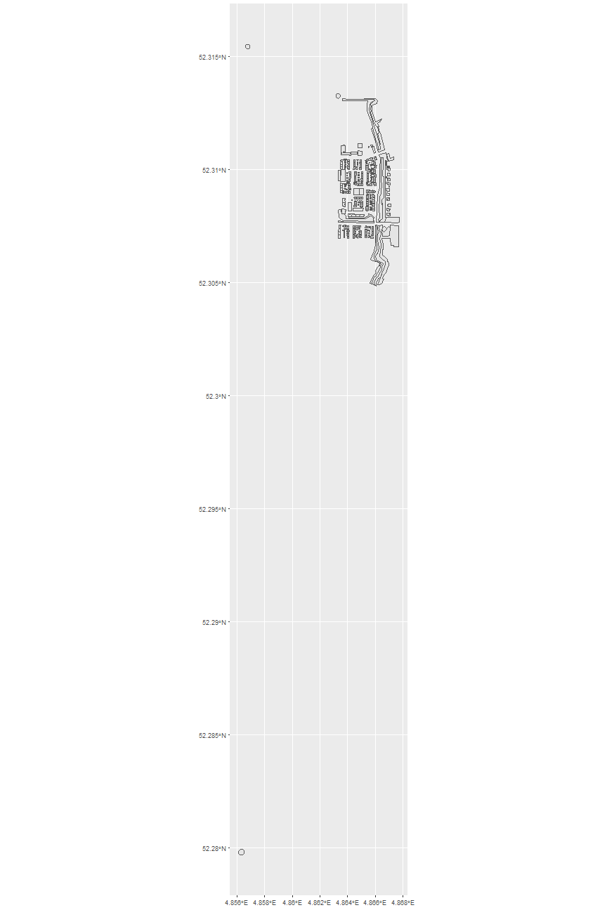
Fine tune the polygons

From the plot in Figure 1 we see that something is wrong. It appears that two polygon features are included (‘round abouts’) that do not belong to this bbox. Therefore we add to each feature its own bbox (in the fields xmin, ymin, xmax and ymax ) so that we can specify exactly which feature we want to keep.


polygons1 = cbind( 
  od$osm_polygons, 
  purrr::map_dfr(st_geometry(od$osm_polygons),st_bbox)
    ) 
setdiff(names(polygons1),names(od$osm_polygons)) # list added fields 
#> [1] "xmin" "ymin" "xmax" "ymax"
polygons2=polygons1 %>% filter(ymax<52.31080 & ymin > 52.3075)

Color the polygons

To color features depending on their function we make a frequency distribution of the character attributes to see which are the interesting one. Because the output is rather bulky we only show the code we used

x= purrr::keep(polygons2,is.character)
st_geometry(x) = NULL
purrr::iwalk(x, function (x1, x2) {
  if (! x2 %in% c('ref.bag', 'osm_id')){
  cat('\n', x2, '\n')
  print(table(x1, useNA = "ifany",dnn=NULL))}
})

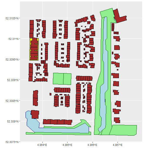
With this information we can color the polygons

ggplot() +
  geom_sf(data=polygons2 %>% filter (natural == 'water'),
          color='darkblue',fill='lightblue') +
  geom_sf(data=polygons2 %>% filter (landuse %in% c('forest', 'grass') ),
          color='darkgreen',fill='lightgreen') +  
  geom_sf(data=polygons2 %>% filter (landuse %in% c('retail') ),
          color='black',fill='yellow') +
  geom_sf(data=polygons2 %>% filter (leisure == 'playground' ),
          color='darkgreen',fill='lightgreen') + 
  geom_sf(data=polygons2 %>% filter (! is.na(building) ),
          color='black',fill='brown')

plot of chunk color-polygons

Figure 2: Open Street Map polygons colored by function

Session Info

This document was produced on 01Jul2020 with the following R environment:

  #> R version 4.0.2 (2020-06-22)
  #> Platform: x86_64-w64-mingw32/x64 (64-bit)
  #> Running under: Windows 10 x64 (build 18363)
  #> 
  #> Matrix products: default
  #> 
  #> locale:
  #> [1] LC_COLLATE=English_United States.1252 
  #> [2] LC_CTYPE=English_United States.1252   
  #> [3] LC_MONETARY=English_United States.1252
  #> [4] LC_NUMERIC=C                          
  #> [5] LC_TIME=English_United States.1252    
  #> 
  #> attached base packages:
  #> [1] stats     graphics  grDevices utils     datasets  methods   base     
  #> 
  #> other attached packages:
  #> [1] stringr_1.4.0 purrr_0.3.4   dplyr_1.0.0   ggplot2_3.3.2 osmdata_0.1.3
  #> [6] sf_0.9-4     
  #> 
  #> loaded via a namespace (and not attached):
  #>  [1] Rcpp_1.0.4.6       highr_0.8          compiler_4.0.2     pillar_1.4.3      
  #>  [5] captioner_2.2.3    class_7.3-17       tools_4.0.2        digest_0.6.25     
  #>  [9] gtable_0.3.0       lubridate_1.7.9    jsonlite_1.7.0     evaluate_0.14     
  #> [13] lifecycle_0.2.0    tibble_3.0.1       lattice_0.20-41    pkgconfig_2.0.3   
  #> [17] rlang_0.4.6        DBI_1.1.0          curl_4.3           xfun_0.15         
  #> [21] e1071_1.7-3        withr_2.2.0        xml2_1.3.2         httr_1.4.1        
  #> [25] knitr_1.29         generics_0.0.2     vctrs_0.3.1        classInt_0.4-3    
  #> [29] grid_4.0.2         tidyselect_1.1.0   glue_1.4.1         R6_2.4.1          
  #> [33] rmarkdown_2.3      sp_1.4-2           farver_2.0.3       magrittr_1.5      
  #> [37] scales_1.1.0       htmltools_0.4.0    ellipsis_0.3.0     units_0.6-6       
  #> [41] rvest_0.3.5        colorspace_1.4-1   KernSmooth_2.23-17 stringi_1.4.6     
  #> [45] munsell_0.5.0      HOQCutil_0.1.22    crayon_1.3.4

Han Oostdijk